Vor einiger Zeit haben wir im PRAKLA-SEISMOS Datenzentrum das Verfahren der "Migration mit Hilfe der Wellengleichung" in unser seismisches Programmpaket aufgenommen. Inzwischen ist es unseren Mitarbeitern M. Morawe und J. Lenz gelungen, das anfangs zeitaufwendige Programm so zu optimieren, daß heute für eine Migration nur noch ein Bruchteil der ursprünglich erforderlichen Rechenzeit benötigt wird.

Die dem Verfahren zugrunde liegenden Gedanken sind neu und recht ungewohnt. Darum soll hier versucht werden, eine zusammenhängende und möglichst verständliche Darstellung des Verfahrens aus den theoretischen Grundlagen zu entwickeln.

Um die wesentlichen Zusammenhänge zu verdeutlichen, machen wir zunächst einige vereinfachende Annahmen :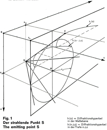

The Working of
Wave Equation Migration
In our PRAKLA-SEISMOS Report 1/76 Mr. W. Houba first reported on the migration procedure using the wave equation. In the Report 2/76, M r. H. Rist traced this procedure with respect to its consumption of computing time and its dependence on the depth step width. In the following article the working of wave equation migration is outlined in detail by means of a theoretical example.

Some time aga we included "wave equation migration" in our Data Centre's seismic program package. In the meantime our colleages M. Morawe and J. Lenz have succeeded in optimizing the initially time-consuming program in such a way that today only a fraction of the originally required computing time is needed.

The concept for this procedure is new and rather unusual. We shall therefore attempt here to give a non-mathematical description. To outline the essential interrelations we make at first three simplifying assumptions:

1. We restrict ourselves to two spatial dimensions, the line direction (x) and the depth (z). The third dimension is to represent clearly the progress in time.
2. We assume ta-times for the processing of seismic data.
3. We consider for this example a constant velocity of v = 2000 m/s. (In areal case, of course, true seismic velocities are considered by the program). Therefore, depths and times can be measured in the 'same scale, for at v = 2000 m/s the double traveltime in ms is equal to the depth in m.

In seismic surveys, a wave field in the subsurface is generated by an energy source e. g. explosives or airguns. A wave field consists of a number of propagating waves which are refracted, reflected and superimposed. Every single wave is a periodic function of space and time, progressing independently of the superimposed waves. The amplitude at a certain point and at a certain time in the wave field is the sum of all amplitudes of single waves appearing at this point.

The spatial and time dependence of the amplitudes w of a wave field can be represented mathematically as a function of the form w = w (x, z, t), see assumption 1. Though there is a close relationship between depth z and traveltime t, we want to regard z and t as independent coordinates in a three-dimensional rectangular system.

Digital data processing requires that a finite sampling (grid) is introduced: x can only adopt values which are multiples of the subsurface point spacing Δx, t can adopt only those values which are multiples of the sampling rate Δt, the same applies for z because of assumption 3.

In recording a seismic line we measure at the earth's surface. At the depth z = 0 along the line direction x we record the amplitudes w as a function of the time t. Considering assumption 2, the x,t-plane in the coordinate system represents nothing else but the time domain in which the seismic section is located. w = w (x, 0, t) is thus the measured time section.

1. Wir beschränken uns auf zwei räumliche Dimensionen, die Profilrichtung (x) und die Tiefe (z). Die dritte Dimension (t) soll der anschaulichen Darstellung des zeitlichen Ablaufes vorbehalten bleiben.
2. Wir setzen für die Bearbeitung der seismischen Daten to-Zeiten voraus.
3. Wir nehmen eine konstante Geschwindigkeit von v = 2000 m/s an. Deshalb lassen sich Tiefen und Zeiten im gleichen Maßstab messen. (Bei v = 2000 m/s ist die doppelte Laufzeit in Millisekunden gleich der Tiefe in Metern). Die tatsächlich ermittelten seismischen Geschwindigkeiten werden im Programm selbstverständlich berücksichtigt.

Bei seismischen Messungen wird durch eine Energiequelle (Sprengladung, Luftpulser usw.) im Untergrund ein Wellenfeid erzeugt. Es besteht aus einer Vielzahl von Wellen, die sich ausbreiten, gebrochen und reflektiert werden und die sich vielfältig überlagern. Jede Einzelwelle ist ein räumlich und zeitlich periodischer Vorgang, der unabhängig von den überlagernden Wellen abläuft. Die Amplitude an einer bestimmten Stelle und zu einer bestimmten Zeit im Weilenfeld ist die Summe aller Amplituden der an dieser Stelle in Erscheinung tretenden Einzelwellen.

Die räumliche und zeitliche Abhängigkeit der Amplituden w eines Wellenfeldes läßt sich mathematisch als Funktion in der Form w = w (x, z, t) darstellen (siehe Annahme 1). Obwohl zwischen der Tiefe z und der Laufzeit t ein enger Zusammenhang besteht, wollen wir z und t als unabhängige Koordinaten in einem dreidimensionalen rechtwinkeligen Koordinatensystem betrachten.

Die digitale Datenverarbeitung erfordert, daß wir ein Raster einführen: x kann nur Werte annehmen, die ein Vielfaches des Untergrundpunktabstandes Δx sind, t nur solche, die ein Vielfaches der Sampling Rate Δt darstellen, und dasselbe gilt für z wegen der Annahme 3).

Bei der Aufnahme eines seismischen Profiles messen wir an der Erdoberfläche - also in der Tiefe z = 0 - entlang der Profilrichtung x Amplituden w in Abhängigkeit von der Zeit t. Beachten wir die Annahme 2), so stellt die x, t-Ebene im Koordinatensystem nichts anderes dar als den Zeitbereich, in dem die gemessene seismische Sektion liegt. w = w (x, 0, t) ist also die gemessene Zeitsektion. Um die Zusammenhänge noch besser zu verstehen, betrachten wir Figur 1. S sei in der x, z-Ebene ein Punkt im Untergrund mit den Koordinaten X_s und z_s, z.B. ein Punkt einer geologischenStörungskante.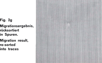

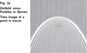
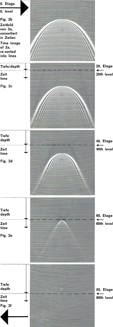
Zur Zeit t = 0 beginnt S eine Welle auszusenden (ausgelöst durch einen auf S treffenden seismischen Impuls), das bedeutet, daß sich um S in der x, z-Ebene eine Welle mit kreisförmiger Wellenfront ausbreitet. Zur Zeit t = t_o habe die WeIlenfront den Radius r = r_o erreicht. Mit fortschreitender Zeit wird ihr Radius immer größer. Die Ausbreitung der Weilenfront wird im x, z, t-Koordinatensystem durch einen Kreiskegel dargestellt, dessen Spitze in S liegt und dessen Achse parallel zur t-Achse verläuft.

Der Wellenfrontkegel schneidet die Meßebene in der uns wohlbekannten Diffraktionshyperbel. Die Diffraktionshyperbel ist also das "Zeitbild" des diffraktierenden Punktes S, der im Tiefenbereich liegt. Der Scheitel T der Diffraktionshyperbel hat die Koordinaten x = x_s, z = 0 und t = Z_s wegen unserer Annahme 3).

Bei seismischen Messungen gilt unser Interesse nicht eigentlich dem gemessenen "Zeitbild", sondern vielmehr den strahlenden (reflektierenden) Punkten selbst, die, wie in dem betrachteten Beispiel der Punkt S, im Tiefenbereich liegen. Für das Migrationsverfahren ergibt sich daraus die Aufgabe, aus dem "Zeitbild" das "Tiefenbild" zu bestimmen. Der Ausdruck " Migration" (= Auswanderung, vom lateinischen migrare = wandern), der bei früher angewandten Methoden berechtigt war, verliert hier seinen ursprünglichen Sinn.

Den Schlüssel zur Lösung dieser Aufgabe stellt die WeIlengleichung dar. Jede Einzelwelle, und damit unser ganzes Wellenfeld, gehorcht der Wellengleichung. Die Weilengleichung ist eine partielle Differentialgleichung, in der die zweiten Ableitungen nach den räumlichen Koordinaten und nach der Zeit vorkommen. Aus einem Teil des Weilenfeldes kann mit Hilfe der Wellengleichung das gesamte Wellenfeld für alle Tiefen (bis zum Bearbeitungsende der seismischen Sektion) berechnet werden. DER UNS BEKANNTE TEIL DES WELLEN FELDES IST DIE GEMESSENE STAPELSEKTION bei z = O.

Die Berechnung des Wellenfeldes geht etagenweise vor sich. Wir berechnen zunächst aus der Stapelsektion w (x, 0, t) das Wellenfeld für die Tiefe z = Δz. Das Ergebnis lautet: w (x, Δz, t). Es entspricht einer Zeitsektion, die in der Tiefe Δz gemessen werden könnte, wenn man alle Geophone in Bohrlöcher der Tiefe Δz versenkt hätte. Von der ersten Etage rechnet man dann weiter zur zweiten Etage in der Tiefe z = 2 Δz usw. bis zum Bearbeitungsende. Für jeden Rasterpunkt im x, z, t-Koordinatensystem wird der zugehörige Amplitudenwert errechnet und somit das gesamte Wellenfeld bestimmt.

In der an der Oberfläche gemessenen Zeitsektion erfassen wir diejenigen Wellen, die aus dem Untergrund zur Erdoberfläche zurückkehren, und nur die nach oben gerichteten Wellen sind für unsere Zwecke von Interesse.

Bei der etagenweisen Berechnung des Wellenfeldes werden die aufwärts laufenden Wellen bis zu ihrem Ausgangspunkt zurückverfolgt: Im Beispiel des strahlenden Punktes (Figur 1) wird der nach oben laufende Teil der kreisbogenförmigen Wellenfront beim Herunterrechnen mit zunehmender Tiefe auf immer kleinere Radien zurückgeführt. Bei Erreichen der Tiefe z = Z_s ist die kreisförmige Wellenfront auf den Radius r = 0 reduziert, das heißt in den Punkt S selbst "fokussiert", und dieser Punkt S ist genau das, was wir suchen: Das Migrationsergebnis.

Zusammenfassend läßt sich die Migration mit der Weilengleichung in der Formel ausdrücken:

und das heißt nichts anderes, als daß die im Zeitbereich gemessene Sektion in den Tiefenbereich übergeführt wird.

Für die etagenweise Bestimmung des Wellenfeldes auf dem Computer ist es erforderlich die Eingabedaten zunächst in Zeilen anzuordnen. Die Bildfolge der Figur 2 zeigt für das Beispiel eines strahlenden Punktes einige Schritte, wie sie tatsächlich im Programm ablaufen.

Figur 2a ist das Zeitbild des strahlenden Punktes in Spuren. In Figur 2b ist die Umsortierung in Zeilen erfolgt, wir haben also die nullte Etage vor uns. Die folgenden Figuren 2c, 2d, 2e und 2f zeigen die 20., 40., 60. und 80. Etage. Wir sehen, daß der bereits fertig migrierte Tiefenbereich immer breiter, der noch zu migrierende Zeitbereich immer schmaler wird. Wir erkennen auch, daß sich die Diffraktionshyperbel im Scheitelbereich immer stärker krümmt und daß der Scheitel selbst immer dichter an die Grenze zwischen Tiefen-und Zeitbereich heranrückt, was aus der Figur 1 verständlich wird.

Abschließend werden die Zeilen des Tiefenbereichs wieder in Spuren rücksortiert (Fig. 2g) und für die Abspielung auf Band ausgegeben.

Wir haben den Migrationsprozeß für einen einzelnen Punkt beschrieben. In der Praxis läuft der Migrationsprozeß in gleicher Art ab für die vielen Punkte, aus denen sich die geologische Struktur im Untergrund "zusammensetzt".

In order to make our considerations more plausible, we regard figure 1. S (in the x, z-plane) is some point in the subsurface with the coordinates X_s and z_s, for instance a point on a geological fault. At the time t = 0 a wave is emitted at S (released by a seismic pulse that hits S), that means, a circular wave front propagates around S in the x,z-plane. At the time t = t_o the wave front reaches the radius r = r_o. With progressing time the radius becomes greater and greater. The propagation of the wave front is represented in the x, z, t coordinate system by a circular cone whose peak is located at Sand whose axis runs parallel to the t-axis.

The wave front cone cuts the survey plane in the diffraction hyperbola which is weil known to us. The diffraction hyperbola is thus the "time image" of the diffracting point S which is located in the depth domain. Vertex T of the diffraction hyperbola has the coordinates x = X_s, Z = 0, and t = Z_s because of our assumption 3.

In seismic surveys our interest is not only concentrated on the measured "time image", but on the reflecting points which - as in our example point S - are located in the depth domain. The migration procedure has thus the task of determining the "depth image" from the "time image". The term "migration", correctly used in previously applied methods, loses here its original sense.

The key to the solution of this problem is the wave equation. Every single wave, and thus our whole wave field, satisfies the wave equation. The wave equation is a partial differential equation involving second derivatives with respect to space and time coordinates. From a part of the wave field, the whole wave field can be computed for all depths (up to the processing end of the seismic section) by means of the wave equation. The part of the wave field known to us is the measured stacked section at z = 0.

The computation of the wave field is carried out in a depth step method. We first calculate the wave field for the depth z = Δz from the stacked section w (x, 0, t). The result is: w (x, Δz, t). It corresponds to a time section which would have been measured if all geophones were placed in boreholes at the depth Δz. From the first level we calculate downwards to the second level at the depth z = Δz and continue doing this up to the processing end. For every grid point in the x, z, t-coordinate system, the corresponding amplitude value is calculated, thus determining the whole wave field.

In the time section measured at the surface we detect those waves which return from the subsurface to the earth's surface. Only the upward waves are of interest for our purposes.

In the depth step computation of the wave field, the upward waves are traced back to their source. In the example of the radiating point (fig. 1) the upward part of the circular wave front is reduced in the progressive downwards calculation to an always smaller radius with increasing depth. On reaching depth z = Z_s the circular wave front is reduced to the radius r = 0, that means it is "focussed" in the point S itself, and this point is exactly the wanted migration result.

Migration using the wave equation can be summarized in the following formula:

That simply means that the section measured in the time domain is transformed to the depth domain.

For the depth step determination of the wave field using the computer it is necessary to have the input data arranged in lines. The chart in figure 2 shows, for the example of a radiating point, several steps as they are realized in the program.

Figure 2a is the time image of the radiating point in traces. In figure 2b a re-sorting into lines has been carried out; the figure shows the Oth level. The following figures 2c, 2d, 2e, and 2f show the 20th, 40th, 60th and the 80th level. We notice that the already migrated depth domain becomes broader, whereas the time domain becomes more narrow. We also notice that the diffraction hyperbola bends more and more near the vertex, and that the vertex itself approaches the boundary between depth-and time domain, as we can derive from figure 1 as weil.

Finally, the lines of the depth domain are again re-sorted into traces (fig. 2g) and output on tape for display.

We described the migration procedure for one single point. In practice, migration runs in the same way for the many points which "compose" the geological structure in the subsurface.